Splitting prefill and decode onto separate GPU pools turns the KV cache from local state into data that has to be routed, moved, and restored. Moving it once turns out to be cheap: in a worked example of a 70B-class coding agent on B200s, handing a 32K-token prompt’s KV from prefill to decode adds about 5% to time to first token over 400 Gb/s RDMA, even without overlap. What is hard is keeping KV reusable. Reuse pays off enormously, since session reuse alone cuts the agent’s prefill work about 24×, but stored KV competes for GPU memory, the resource that already limits decode. Disaggregation adds a second difficulty: prefix hits now depend on routing across two pools, and the newest copy of each session sits on the decode side, where pulling it back every turn costs more as the conversation grows. The upshot is that for any given set of GPUs, caching choices (session reuse, affinity, memory tiers, KV format) determine the traffic it can serve far more than the decision to disaggregate does.
Contents
- 1 Introduction
- 2 Prefill and decode: two phases with opposite bottlenecks
- 3 The KV cache: the state that links the two phases
- 4 Prefix caching: reusing KV across requests
- 5 Session caching: reusing KV across turns
- 6 Co-located serving and its limit: prefill–decode interference
- 7 Disaggregation: splitting prefill and decode into separate pools
- 8 The price of the split: moving KV from P to D
- 9 Caching across two pools: prefix and session reuse after the split
- 10 From analysis to deployment: sizing the pools and deciding whether to split
- 11 Looking ahead: more splits and KV as a cluster resource
- 12 Conclusion: get the cache design right first
- References
Notation and acronyms
| Term | Meaning |
|---|---|
| P, D | Prefill and decode: the two phases, or the worker pools that run them |
| KV cache | The keys and values every token produces at every attention layer |
| TTFT | Time to first token |
| TPOT | Time per output token, averaged over a request’s output after the first token |
| ITL | Inter-token latency: each individual gap between consecutive output tokens |
| GQA | Grouped-query attention: several query heads share one KV head |
| MLA | Multi-head latent attention: caches one compressed latent vector per token |
| MoE | Mixture of experts |
| TP | Tensor parallelism |
| HBM | High-bandwidth memory on the GPU |
| RDMA | Remote direct memory access: the NIC reads and writes GPU memory directly |
| NIXL | NVIDIA Inference Xfer Library, the transfer library vLLM and Dynamo use for KV handoffs |
| BF16, FP8, NVFP4 | 16-bit, 8-bit, and 4-bit number formats (NVFP4 costs about 4.5 bits per value with its scales) |
1 Introduction
1.1 Three caches, two ways to deploy them
In LLM serving, “the cache” can mean three different things.
- The KV cache is the attention state a model builds while it reads a prompt.
- The prefix cache lets a second request reuse that state when it starts with the same tokens.
- The session cache keeps a conversation’s state alive from one turn to the next.
All three are usually discussed as memory optimizations inside a single GPU server, and on a single server that framing works.
It stops working once prefill and decode run on separate machines. The KV cache is then something one pool of GPUs produces and another pool consumes, so it has to be identified, located, moved, leased, and eventually restored. Prefix caching, already a routing problem once a service runs several replicas, now spans two pools, and session caching turns into a question of which machine holds the newest copy of a conversation.
This post builds the three caches up from first principles. It then shows what happens to each of them in the move from a co-located deployment to a disaggregated one. Along the way it puts numbers on the trade-offs, to show which ones dominate for a given workload.
1.2 The running example: a coding agent on a shared repository
The post uses one workload throughout: an internal coding agent that an engineering team runs against a shared repository.
Every agent session starts from the same material:
- a system prompt and tool schemas (about 3,500 tokens);
- a snapshot of the repository’s most important files (about 28,500 tokens).
That gives a 32,000-token shared prefix, identical for every session working on the same commit. The user then adds a task of about 100 tokens.
From there, the agent loops. In each step the model emits a tool call of about 150 tokens (say, “run the failing test”), the tool returns about 1,500 tokens of output, and the next step begins with the entire history as its prompt. Each step is therefore one prefill (mostly the new tool output) followed by one short decode (the next tool call). A typical task takes 20 steps, so by the last step the prompt is about 63,000 tokens long.
| Component | Assumption |
|---|---|
| Model | 70B-class dense transformer with grouped-query attention: 80 layers, 64 query heads, 8 KV heads, head dimension 128, about 141 GB of BF16 weights |
| GPU | NVIDIA B200 as configured in DGX B200: 180 GB HBM3e and 8 TB/s memory bandwidth per GPU, about 2.25 PFLOPS dense BF16 |
| Interconnect | Fifth-generation NVLink (1.8 TB/s bidirectional per GPU) inside a node; one 400 Gb/s ConnectX-7 NIC per GPU between nodes |
| Node | 8 GPUs, 2 TB of host memory, about 30 TB of local NVMe |
| Serving instance | Tensor parallelism of 2 (TP=2): two GPUs per instance, leaving about 200 GB for KV after weights and workspace |
| Compute efficiency | Prefill estimates assume 60% of peak dense BF16 throughput |
Note. All numbers below are back-of-envelope estimates under these assumptions. They are meant to show orders of magnitude and relative costs, not to predict what any particular stack will measure. Implementation details reflect the vLLM, NVIDIA Dynamo (v1.5.1), and SGLang documentation as of October 2026.
2 Prefill and decode: two phases with opposite bottlenecks
Every request runs in two phases.
- Prefill (P) processes the whole prompt in one forward pass and produces the attention keys and values for every prompt token at every layer.
- Decode (D) then generates output tokens one at a time. Each new token attends to everything before it and appends its own keys and values.
The two phases stress the hardware in opposite ways, and the roofline model explains why.
2.1 Compute-bound or memory-bound: the ridge point
A GPU’s ridge point is its peak FLOP rate divided by its memory bandwidth. For a B200 that is about 2.25 PFLOPS ÷ 8 TB/s ≈ 281 FLOPs per byte; an H100 SXM sits at about 295. Any kernel that performs fewer FLOPs per byte of memory traffic than the ridge point is limited by memory bandwidth, not by compute.
2.2 Linear layers: intensity equals tokens per pass
The QKV and output projections and the MLP hold almost all of a model’s parameters. Excluding the attention-score computation, a forward pass with T tokens through a model with N parameters performs about 2·T·N FLOPs and reads the 2·N bytes of BF16 weights once. The arithmetic intensity is therefore about T FLOPs per byte.
- Prefill.
Tis the prompt length: thousands of tokens, far above the ridge point. Prefill is compute-bound. - Decode.
Tis the batch size, because each sequence contributes one token per step. The linear layers stay memory-bound until a batch reaches roughly 300 sequences, and in practice KV capacity caps the batch long before that.
2.3 Decode attention: intensity equals the GQA group size
Attention during decode is worse. Each sequence reads its own KV history, and that read cannot be shared across the batch. For every key/value element loaded, the work is proportional to the number of query heads that share that KV head, the GQA group size G. Decode attention therefore runs at roughly G FLOPs per byte, no matter how large the batch is.
The example model has 64 query heads and 8 KV heads, so G = 8. Its decode attention is deeply memory-bound.
Multi-head latent attention (MLA), introduced in DeepSeek-V2 and used in DeepSeek-V3 and several later models, is the notable exception. MLA caches one compressed latent vector per token instead of per-head keys and values. In its absorbed form, where the up-projection matrices are folded into the query and output projections, attention runs directly on that latent. Every query head reads the same vector per token, so the effective group size equals the number of query heads on the GPU, which is 128 for DeepSeek-V3 when attention runs data-parallel with every head on one GPU. That raises decode attention’s intensity to within reach of the ridge point.
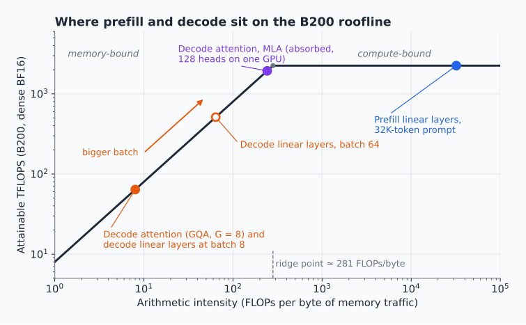
Where each kind of work sits on the B200 roofline. Decode attention with GQA stays memory-bound at any batch size; batching only helps the decode linear layers.
The compute-bound side has its own kernel-level story: the earlier post FlashAttention-3 on Hopper walks through how an attention kernel keeps the tensor cores busy.
2.4 Putting numbers on both phases
Prefill. Prefilling the first request (the 32,000-token prefix plus the 100-token task) takes about 5.9 × 10¹⁵ FLOPs. Attention contributes about 23% of that, because its cost grows quadratically with prompt length. At 60% of peak on two B200s, the prefill takes about 2.2 seconds.
Decode. Every decode step must stream essentially all ~141 GB of weights, split across the two GPUs. At the full 16 TB/s of combined HBM bandwidth, that takes at least 8.8 ms before a single byte of KV is read. A session with 48,000 tokens of context then adds about 15.7 GB of KV, or roughly 1 ms of extra reads per step. With eight such sessions in a batch, the KV reads (about 126 GB) nearly match the weight reads, and the step’s memory traffic alone takes about 17 ms.
At long context, KV reads rival the weight reads with only a handful of sequences in the batch, and dominate beyond that.
2.5 Latency targets and goodput
The two phases map onto three latency metrics:
- Time to first token (TTFT) is dominated by queueing plus prefill.
- Time per output token (TPOT) is dominated by the decode step time. It averages over a request’s output tokens after the first.
- Inter-token latency (ITL) measures each individual gap between consecutive tokens, so its tail captures stalls that TPOT averages away.
A useful system-level metric is goodput, as defined by DistServe: the highest request rate at which a required fraction of requests meets both its TTFT and TPOT targets. Much of this post is about what threatens one target when the system is optimized for the other.
Takeaway. Prefill is limited by compute and decode by memory bandwidth, and at long context the KV cache, not the weights, dominates decode traffic.
3 The KV cache: the state that links the two phases
3.1 What it holds and how big it gets
During prefill, every layer computes a key vector and a value vector for every token. Decode needs all of them for every subsequent step. Recomputing them at every step would mean re-running the projections over the entire history for each new token, so the engine stores them instead. That store is the KV cache.
For standard multi-head or grouped-query attention, its size per token is (the factor of 2 counts keys and values):
| Model shape | Attention | KV per token (BF16) |
|---|---|---|
| 8B-class (32 layers, 8 KV heads, head_dim 128) | GQA, G = 4 | 128 KiB |
| The example 70B-class model (80 layers, 8 KV heads, head_dim 128) | GQA, G = 8 | 320 KiB |
| 70B-class with full multi-head attention (64 KV heads) | MHA | 2.5 MiB |
| DeepSeek-V3 shape (61 layers, 512-dim latent plus 64-dim RoPE key) | MLA | ~68.6 KiB |
Applied to the running example, the shared 32,000-token prefix is about 10.5 GB of KV. A session at step 20, with about 63,000 tokens, holds about 20.8 GB. That is more than a tenth of the KV budget of a two-GPU instance, for a single conversation.
Quantized KV is the first lever on capacity. FP8 halves these sizes, and 4-bit formats such as NVFP4 roughly quarter them, plus some overhead for scales. The format matters beyond capacity. Most systems copy KV to host memory, write it to SSD, or send it over the network in the same format it has in HBM. Everything later in this post that moves KV therefore benefits from a smaller format, and every component that moves KV must agree on that format.
3.2 Paged blocks: the unit every cache operates on
Modern engines do not store each sequence’s KV contiguously. Following PagedAttention, they carve KV memory into fixed-size blocks (pages), commonly 16 tokens each, though some attention backends require larger pages. They keep a per-sequence block table that maps logical positions to physical blocks.
Paging nearly eliminates memory fragmentation, since the waste is limited to each sequence’s partially filled last block, and it makes sharing cheap. If two sequences start with the same tokens, both block tables can point to the same physical blocks, with reference counts deciding when a block can be freed. Prefix caching, session caching, and KV transfer all operate on these blocks.
3.3 How parallelism shards or replicates the KV
Tensor parallelism with GQA. The KV cache is sharded by KV head. In the example’s TP=2 instance, each GPU holds 4 of the 8 KV heads, which is half of every block.
Tensor parallelism with MLA. There is only one latent vector per token, so it cannot be split by head and is replicated on every TP rank instead. vLLM’s design notes state this explicitly (NIXL push-mode design). This is one reason MLA models usually prefer data-parallel attention over tensor-parallel attention; DeepSeek’s own production deployment runs MLA data-parallel in both phases.
Hybrid models. Models that mix full attention with other layer types carry different state in those layers. Sliding-window layers keep only a bounded window of KV, and linear-attention or state-space layers keep a fixed-size recurrent state instead of per-token KV. That state has to travel with the KV whenever a sequence moves.
3.4 Capacity: the real limit on decode batch size
The KV budget directly bounds how much work a decode instance can hold.
- In BF16, the example instance’s ~200 GB holds about 9 step-20 agent sessions.
- In FP8, it holds about 19.
- With the 32,000-token prefix stored once and shared across sessions, it holds about 18 in BF16 and 37 in FP8.
Batch size, and therefore decode throughput, is set by these numbers long before compute runs out. Every technique in the rest of this post either saves KV memory, avoids recomputing KV, or moves KV to where it’s needed.
3.5 What 4-bit KV changes
NVFP4 stores each value in 4 bits and adds one FP8 (E4M3) scale per 16-value block, plus one FP32 scale per tensor. That costs about 4.5 bits per value, or about 28% of BF16 (NVIDIA’s NVFP4 introduction). Applied to the running example’s KV cache:
| Quantity | BF16 | FP8 | NVFP4 |
|---|---|---|---|
| KV per token | 320 KiB | 160 KiB | ~90 KiB |
| Step-20 session | ~20.8 GB | ~10.4 GB | ~5.8 GB |
| Step-20 sessions per TP=2 instance | ~9 | ~19 | ~34 |
| First-request KV handoff over two 400 Gb/s NICs | ~117 ms | ~58 ms | ~33 ms |
| Decode attention intensity (G = 8) | ~8 FLOPs/byte | ~16 FLOPs/byte | ~28 FLOPs/byte |
Three things follow.
- Capacity and decode speed improve together. Even at about 28 FLOPs per byte, decode attention stays far below the ridge point, so every byte saved shortens the decode step. The consolidated decode instance in Section 10, which needs about 37 ms per step with BF16 KV, would need about 17 ms with NVFP4 KV, without any special kernel.
- Everything that moves KV gets cheaper by the same factor. Handoffs, offloads to host memory, and restores from a shared tier all shrink to about 28% of their BF16 size.
- The costs are accuracy and compatibility. Four bits lose more information than eight, so accuracy has to be validated for each model and workload, especially at long context. The attention kernel must read the 4-bit values and their scales, and every component that stores or moves KV must agree on the layout: block scales stored inside each paged block travel with it, while per-tensor scales must match on both sides of a transfer. Support varies across engines and attention backends, so it needs to be confirmed before capacity is planned around it.
Takeaway. KV capacity, not compute, sets how many sequences a decode instance can serve; smaller KV formats and block sharing are the first levers.
4 Prefix caching: reusing KV across requests
4.1 How engines find a matching prefix
Two requests that begin with the same tokens produce identical KV for that shared beginning, because under causal attention a token’s keys and values depend only on that token, its position, and the tokens before it. Prefix caching exploits this by keeping KV blocks around after a request finishes and handing them to any later request whose prompt starts the same way.
Engines typically find matches in one of two ways.
Hash chains (vLLM). Each full block is identified by a hash of three things: its parent block’s hash, the tokens in the block, and extra keys such as a LoRA adapter ID or multimodal input hashes (vLLM prefix caching design). Because each hash includes its parent’s, one block hash identifies the entire prefix up to that point. Matching means hashing the incoming prompt block by block and looking up each hash until the first miss.
Radix trees (SGLang). RadixAttention stores token sequences in a radix tree and matches at token granularity, evicting least-recently-used leaves. SGLang’s HiCache extends the same tree into host memory and external storage (LMSYS blog).
A few details matter in practice:
- Only full blocks are cacheable in a block-hashed design. With 16-token blocks, the example’s 32,000-token shared prefix fills exactly 2,000 blocks, so all of it can be shared. Had it been 32,010 tokens long, the last 10 tokens would fall into a block that also contains each session’s own task tokens, and every session would recompute them.
- “Finished” does not mean “gone.” When a request ends, its blocks drop to a reference count of zero and move to an evictable pool, but their contents stay valid until the memory is needed. The cache’s effective size is “all KV memory not currently in use,” and eviction is usually LRU.
- Isolation has to be requested explicitly. A cache hit is measurably faster than a miss, so a cache shared across tenants leaks information through timing. vLLM lets a request carry a
cache_saltthat is mixed into the first block’s hash, so only requests with the same salt can share blocks.
4.2 The payoff: from a 2.2-second prefill to one weight pass
The first session on a given commit pays the full ~2.2-second prefill. Every later session on that commit finds the 32,000-token prefix already cached and prefills only its 100-token task. A 100-token pass is too small to be compute-bound; it costs roughly the ~9 ms it takes to stream the weights. TTFT collapses from seconds to that pass plus queueing and scheduling overhead.
4.3 Why one changed token breaks reuse
Prefix caches fail safe: a mismatch is just a miss, never a wrong answer. But they are unforgiving, because a change at token position p invalidates the block containing p and every block after it. In the coding agent, any of these would destroy reuse for everyone:
- a timestamp or request ID near the top of the system prompt;
- tool schemas serialized in a nondeterministic order;
- repository files concatenated in filesystem order rather than a stable sorted order;
- a frequently changing file (a lockfile, a changelog) placed early in the repository context.
Design rule. Order the prompt from most stable to most volatile: system prompt, then tool schemas, then repository context sorted by how rarely each file changes, then the task.
4.4 With multiple replicas, caching becomes routing
Prefix caching is local to each engine. With N replicas behind a load balancer that ignores the cache, a request whose prefix is cached on only one replica lands there only about 1/N of the time. A hot prefix eventually gets cached on every replica, at the cost of N cold prefills and N copies; long-tail prefixes and per-session state never do. Making the cache work across a fleet requires the router to know where each prefix lives and to send requests there.
Public APIs make this visible. OpenAI’s prompt-caching documentation describes routing each request to a machine based on a hash of the prompt’s initial prefix, combined with an optional user-supplied prompt_cache_key, so that requests sharing a prefix land on the machine that has it cached (OpenAI docs).
Inside a self-hosted cluster, a cache-aware router needs two things.
A global index. Engines such as vLLM can publish KV events whenever blocks are stored or evicted, and the router maintains an index of which worker holds which blocks. NVIDIA Dynamo’s KV router uses these events to track which blocks each worker has cached.
A cost function that balances hits against load. Always routing to the replica with the longest match concentrates hot prefixes on one machine until its queue destroys the TTFT that the cache hit saved. Current Dynamo releases score each worker like this (Dynamo routing concepts):
adjusted_prefill_blocks = max(0, active_prefill_blocks + incoming_prompt_blocks - overlap_credit_blocks)
potential_decode_blocks = active_decode_blocks + incoming_active_blocks
cost = prefill_load_scale × adjusted_prefill_blocks + potential_decode_blocks + active_request_blocks
The prefill term counts the prompt work the worker would face, including prefills already assigned to it, minus a credit for the request’s cached prefix. Hits in GPU memory, host memory, disk, or a shared cache each earn a configurable credit, and the GPU-memory credit can decay when a cache-rich worker already carries too much prefill work, which directly counters the hot-spot problem. The decode term is the KV the worker would hold if it accepted the request, and the optional active-request term is off by default. The router picks the lowest-cost eligible worker.
Takeaway. Prefix caching pays off across a fleet only when the router knows where each prefix lives and balances cache hits against load.
5 Session caching: reusing KV across turns
5.1 Why agent loops depend on session reuse
Prefix caching shares state across different requests. Session caching keeps state for one conversation across its turns. In a short chat, that is a convenience. In agent loops, it decides whether the system is viable, because each step’s prompt is the previous step’s prompt plus a little more.
Here is the coding agent’s 20-step task under three caching regimes. The numbers cover prefill compute only, excluding queueing; one instance-second is one TP=2 instance busy for one second.
| Caching regime | Tokens prefilled over the task | Prefill compute (TP=2 instance-seconds) | Prefill time at step 20 |
|---|---|---|---|
| None: every step re-prefills its whole prompt | ~956,000 | ~73 | ~5.3 s |
| Shared prefix only: the 32K prefix hits, the trajectory is recomputed each step | ~316,000 | ~30 | ~3.1 s |
| Full session reuse: each step prefills only what was appended since the previous step (~1,650 tokens) | ~31,000 | ~3.1 | ~0.19 s |
Full session reuse cuts prefill work about 24× compared with no caching, and about 10× compared with sharing only the prefix. It is also the only regime in which per-step prefill time grows slowly, from about 0.14 s at step 2 to about 0.19 s at step 20, because only the attention over the longer context gets more expensive. Without it, each step re-prefills an ever-longer prompt and takes markedly longer than the last.
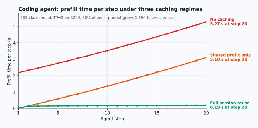
Prefill time per step for the coding agent. Only full session reuse keeps step latency roughly flat as the conversation grows.
5.2 On one engine: prefix caching plus affinity
On one engine, “session caching” needs no special mechanism. The KV of the tokens the model generated in step k lives in the same paged pool as everything else, and its full blocks are hashed and cached like prompt blocks.
When the step k+1 request arrives, its prompt is step k’s prompt plus the generated tool call plus the new tool output. The engine’s prefix cache therefore matches everything up to the new tool output, down to the last full block, provided the client sends back exactly the tokens the model generated.
The only requirement is session affinity: step k+1 has to land on the engine that served step k.
Session reuse breaks when affinity fails or the cached blocks no longer match the new prompt:
- Routing changes. A load balancer moves the session to another replica.
- Eviction. Memory pressure pushes the session’s blocks out of the LRU pool while the agent waits on a slow tool.
- Restarts. The engine is rescaled, upgraded, or crashes.
- Long idle gaps. A human steps away and comes back an hour later.
- History edits. The client strips reasoning traces, re-renders messages through a chat template that tokenizes them differently from how they were generated, or truncates and summarizes old turns. The new prompt then diverges from the cached tokens, and the hash chain breaks at the first difference.
Each failure falls back either to a shorter prefix hit (usually just the shared 32K) or to a full re-prefill. None of them produces wrong output, because the match is by content; Section 9 shows why that guarantee disappears when KV is reused across engines by position.
5.3 Where session KV waits between turns
The gap between turns decides where a session’s KV can afford to wait:
- agent tool calls come back in seconds;
- human chat comes back in tens of seconds to minutes;
- resumed sessions may come back hours or days later.
GPU memory cannot hold many idle 20 GB sessions, so sessions waiting longer than a few seconds need somewhere cheaper:
| Tier | Typical capacity | Idle step-20 sessions it holds (BF16) | Time to bring one back to the GPUs |
|---|---|---|---|
| GPU HBM (one TP=2 instance) | ~200 GB of KV budget | ~9, each displacing active work | already there |
| Host DRAM (x86 node such as DGX B200) | 2 TB per node | ~95 | ~210 ms over PCIe Gen5, assuming ~50 GB/s per GPU |
| Grace CPU memory (GB200) | up to 480 GB of LPDDR5X per Grace CPU, shared by its two GPUs | ~23 | ~40 ms, limited by the Grace CPU’s ~500 GB/s memory bandwidth rather than by NVLink-C2C (900 GB/s bidirectional) |
| Local NVMe | ~30 TB per DGX B200 node | ~1,500 | bounded by aggregate SSD bandwidth |
| Remote or distributed store | effectively unbounded | — | bounded by network bandwidth |
Compare these restore times with recomputing a step-20 session from scratch: about 5.3 seconds. Even the PCIe path restores about 25× faster than recomputation, and the GB200 path about 125× faster. For long sessions, keeping KV is far cheaper than regenerating it, as long as there is somewhere to put it.
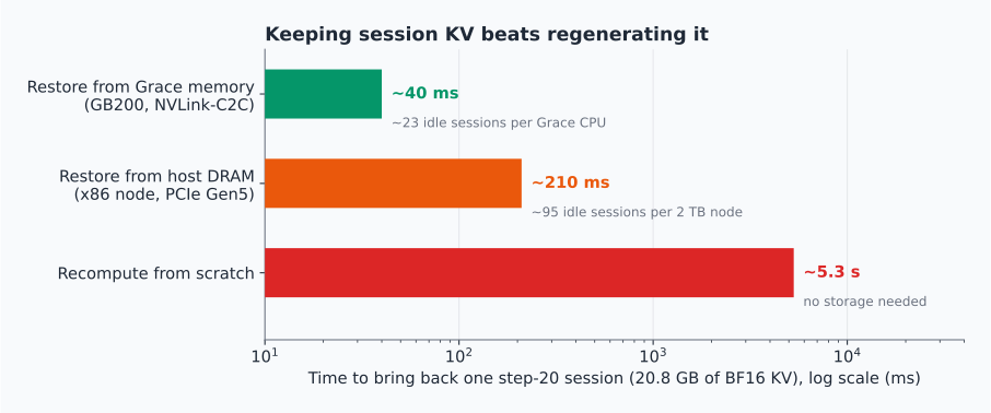
Restoring a step-20 session from a lower memory tier versus recomputing it.
Several systems implement this tiering:
- NVIDIA Dynamo’s KV Block Manager (KVBM) offloads KV blocks through four tiers: G1 (GPU memory), G2 (host memory), G3 (disk), and G4 (object storage) (KVBM configuration reference).
- SGLang HiCache layers GPU, host, and pluggable storage backends (Mooncake, 3FS, NIXL, and others) under its radix tree (HiCache best practices).
- LMCache is a KV caching layer, widely used with vLLM, that can store KV in CPU memory, on local disk, or in remote backends.
- Mooncake Store is a distributed KV cache pool that backs both vLLM and SGLang.
At provider scale the payoff is large. DeepSeek reported that across its V3 and R1 traffic in one 24-hour period, 56.3% of 608 billion input tokens hit its on-disk KV cache (DeepSeek inference system overview).
Takeaway. For agents, session reuse cuts prefill work about 24×, and restoring session KV from a cheaper tier beats recomputing it by 25× or more.
6 Co-located serving and its limit: prefill–decode interference
In a co-located deployment (NVIDIA Dynamo calls it aggregated), each serving instance does both phases. A request arrives, the instance prefills it, the KV stays in that instance’s memory, and the same instance decodes. The instance may span several GPUs through tensor or pipeline parallelism, but logically it handles both P and D.
The appeal is real:
- No transfer. Freshly computed KV is already where decode needs it.
- Short paths. Scheduling, failure handling, and monitoring all stay within one instance.
- Caching is local. Prefix and session caching work through the engine’s own block pool, plus affinity routing at the load balancer.
- Small failure domain. A crash affects only the requests on that instance.
For many deployments, with moderate contexts, moderate concurrency, or relaxed latency targets, this is the right answer.
6.1 How one prefill stalls every decode stream
The trouble starts when both phases share one GPU’s time. Engines use continuous batching, and with chunked prefill enabled (the default in vLLM V1) each step mixes decode tokens from running sequences with prompt tokens from new requests. Prefill tokens are expensive, so they stretch the step, and every decoding sequence in that step waits.
In the coding agent, a decode-only step with eight long sessions takes about 17 ms, all of it memory traffic. Adding prefill tokens to the same step makes the linear layers compute-bound, and the step stretches accordingly. A 512-token chunk roughly doubles the step, a 2,048-token chunk makes it about 7× longer, and an unchunked 32K-token session start freezes every stream for over two seconds. These estimates leave out the chunk’s own attention over the earlier part of its prompt, a cost that grows the deeper into a long prompt the chunk sits.
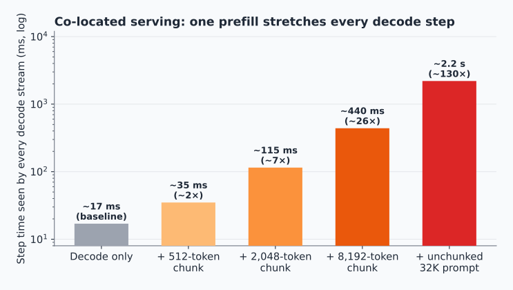
Step time seen by every co-scheduled decode stream when prefill work joins the batch.
6.2 Chunked prefill trades TTFT against TPOT
Chunked prefill splits long prompts into pieces and admits one piece per step alongside the running decodes. Sarathi-Serve formalized this as stall-free batching: every step first schedules all ongoing decodes, then fills the remaining per-step token budget with a prefill chunk. Its authors documented generation stalls lasting several seconds in schedulers that let prefills take priority (Sarathi-Serve, OSDI ‘24). In vLLM, the per-step budget is max_num_batched_tokens.
But chunking only trades one target for the other:
- Large chunks finish prefills quickly, protecting TTFT, but stretch decode steps, hurting TPOT.
- Small chunks protect TPOT but make prefills slower and less efficient. Every chunk re-reads the weights, and every chunk’s attention re-reads all of the prompt’s earlier KV.
A co-located scheduler is therefore always choosing a point on the TTFT–TPOT curve, and long-prompt arrivals keep pushing that point around. Disaggregation exists to remove the trade-off by removing the contention.
Takeaway. Co-located serving is simple and often the right choice, but every prefill taxes every decode stream, and chunking only moves that cost between TTFT and TPOT.
7 Disaggregation: splitting prefill and decode into separate pools
A disaggregated deployment splits the cluster into two pools:
- Prefill (P) workers take new prompts and compute their KV. Depending on the implementation, they may also produce the first output token.
- Decode (D) workers receive that KV and generate the rest of the output.
A request now flows: router → P worker → prefill → KV handoff → D worker → decode.
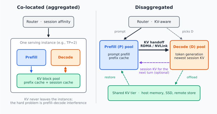
Where the KV cache lives in each deployment style.
7.1 What the split buys
Isolation. Long prompts land only on P, so D’s step time no longer depends on who just submitted a 30K-token prompt. TTFT and TPOT can be tuned independently, with separate batching policies, chunk sizes, and admission rules.
Independent scaling. The P:D ratio becomes a tunable dial. Long-input, short-output traffic needs more P. Many long-running decodes need more D. When the traffic mix shifts during the day, the pools can be resized separately.
Specialization. Each pool can use the parallelism, and even the hardware, that suits its phase:
- DeepSeek serves V3/R1 with prefill units spanning 4 nodes (expert parallelism across 32 GPUs) and decode units spanning 18 nodes (expert parallelism across 144 GPUs). Spreading the experts over more GPUs leaves each decode GPU with only 2 routed experts (versus 9 per prefill GPU), so each expert sees a large enough batch to use the GPU efficiently. The deployment runs on H800 GPUs (DeepSeek inference system overview).
- Splitwise placed each phase on hardware suited to it, including mixed-GPU clusters. It reported up to 1.4× higher throughput at 20% lower cost, or 2.35× more throughput under the same power and cost budgets (Splitwise, ISCA ‘24).
- DistServe framed the goal as maximizing goodput per GPU. It chose parallelism separately for each phase and then replicated instances to match traffic (DistServe, OSDI ‘24).
7.2 What the split costs
- Weights are duplicated. Each pool holds its own complete copy of the model weights.
- The KV must move. Every request’s KV has to get from P to D, and for multi-turn sessions sometimes back again.
- Routing gets harder. The router must understand cache locations, load, and topology for two pools instead of one.
- New failure modes appear. A transfer can fail, time out, or arrive after its lease has expired.
- Layouts must agree. If P and D use different parallel or memory layouts, the KV has to be translated in flight.
- Monitoring expands. Tokens per second is no longer enough; bytes moved, transfer latency, and time spent waiting matter too.
Section 8 covers the transfer, layout, and failure items in detail.
Disaggregation also need not be all-or-nothing. With conditional disaggregation, the router sends some requests through a prefill worker as usual and sends others straight to a decode worker, which runs the prefill locally. In current Dynamo releases the feature is experimental. Its default policy serves a request locally when the effective prompt length (the prompt minus the decode worker’s own cached prefix) is below 2,048 tokens and below 70% of the raw prompt length. Other policies also weigh how busy the prefill workers are, and an optional guard falls back to remote prefill when the decode worker’s KV usage exceeds a configured fraction of its capacity. Dynamo’s documentation positions it for multi-turn and agentic workloads with heavy KV reuse (Dynamo conditional disaggregation).
The trade. Disaggregation is not a switch that makes serving faster. It is a trade: interference isolation and independent scaling in exchange for a distributed KV data plane. Whether the trade pays off is the subject of the next three sections.
8 The price of the split: moving KV from P to D
8.1 How big is the handoff, and how long does it take?
The first request of each coding-agent session produces about 10.5 GB of KV during prefill (the 32,100 tokens at 320 KiB each). With TP=2 on both sides, each GPU holds half of that and can send it over its own NIC using RDMA (remote direct memory access), which lets the NIC read and write GPU memory directly without staging through the CPU. In vLLM, these transfers run through NIXL (NVIDIA Inference Xfer Library), an open-source transfer library from the Dynamo project that runs over UCX and other transport backends.
| Path | Assumed effective bandwidth (per instance) | Time to move 10.5 GB |
|---|---|---|
| NVLink 5 within one NVLink domain (e.g., P and D in the same 8-GPU node) | ~1.8 TB/s (two GPUs × ~900 GB/s per direction) | ~6 ms |
| Two 800 Gb/s RDMA NICs | ~180 GB/s | ~58 ms |
| Two 400 Gb/s RDMA NICs | ~90 GB/s | ~117 ms |
| 100 GbE over TCP, staged through host memory | ~10 GB/s | ~1 s |
The prefill that produced this KV took about 2.2 seconds, so even the 400 Gb/s path adds only about 5% to TTFT, and that is without any overlap. TCP adds almost 50%, which is why production disaggregation runs over RDMA or NVLink.
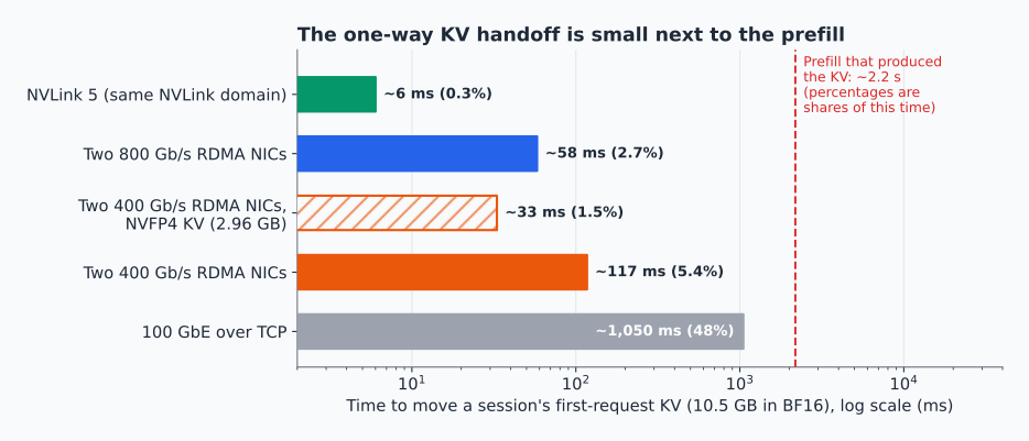
Moving a session’s first-request KV over different links, compared with the prefill that produced it.
A typical agent step produces only about 0.54 GB of new KV (its 1,650 new tokens), so its P→D transfer takes about 6 ms over the same NICs.
8.2 The real cost is exposed latency, not bandwidth
A busy P instance produces KV at its prefill rate times the KV size per token. In the running example that is about 14,700 tokens/s × 320 KiB ≈ 4.8 GB/s, far below the ~90 GB/s that two 400 Gb/s NICs provide. In steady state, the network has plenty of headroom.
What hurts is latency that isn’t overlapped with compute, and per-transfer overhead when prompts are short and their KV is scattered across many small blocks.
That exposed latency has also grown relative to compute. DGX H100 and DGX B200 both give each GPU one 400 Gb/s ConnectX-7 NIC, while dense BF16 throughput per GPU rose from about 989 TFLOPS to about 2.25 PFLOPS. When prefill gets 2.3× faster and the NIC stays the same, an unoverlapped transfer takes 2.3× as large a share of TTFT.
8.3 Which models tolerate the handoff best
A useful figure of merit is how many bytes of KV a model produces per FLOP of prefill compute. Lower is friendlier.
| Model shape | KV per token | Linear-layer FLOPs per token (≈ 2 × active params) | KV bytes per FLOP |
|---|---|---|---|
| 8B dense, GQA | 128 KiB | 1.6 × 10¹⁰ | 8.2 × 10⁻⁶ |
| 70B dense, GQA (the example model) | 320 KiB | 1.4 × 10¹¹ | 2.3 × 10⁻⁶ |
| DeepSeek-V3-style MoE with MLA (~37B active) | 68.6 KiB | 7.4 × 10¹⁰ | 9.5 × 10⁻⁷ |
Two factors make the transfer cheaper relative to the work that produced it:
- Larger models, GQA, and MLA produce less KV per unit of compute.
- Longer prompts help too, because attention FLOPs grow quadratically with prompt length while KV grows only linearly.
Disaggregation therefore pays off most for large models serving long prompts, and least for small dense models serving short ones. DistServe’s evaluation reached a consistent conclusion. On InfiniBand clusters, cross-node KV transfer overhead was negligible. On clusters with weak inter-node bandwidth, the authors placed corresponding pipeline stages of the prefill and decode instances on the same node, so that transfers stayed on NVLink.
8.4 Overlapping the transfer with prefill
There are three main ways to overlap the handoff with compute:
- Layer-wise streaming. Send each layer’s KV as soon as that layer finishes. As long as each layer’s transfer keeps pace with the next layer’s compute, only about 1/L of the transfer is still outstanding when prefill ends. Mooncake pairs layer-wise prefill with streaming KV transfer for this reason (Mooncake, FAST ‘25).
- Chunk-wise streaming. With chunked prefill on P, ship each chunk’s KV as it completes.
- Transfer after completion. Move everything once prefill ends. This is the simplest option and the default in vLLM’s NIXL connector, but it exposes the full transfer time.
8.5 Pull or push: which side holds memory while waiting
vLLM’s NIXL-based connectors support both a pull mode and a push mode, and the choice determines which pool is left holding memory while a handoff is pending.
Pull (the default). The proxy sends P the request with max_tokens=1, and P keeps the resulting blocks under a lease. The lease defaults to 30 seconds and is extended by heartbeats while the request waits in D’s queue. D allocates destination blocks, reads P’s blocks with an RDMA read, and tells P it can release them (vLLM NixlConnector guide).
Push. D registers its pre-allocated block IDs with P, and P writes the KV directly into D’s memory with an RDMA write once it is ready (push-mode design).
The operational difference matters more than the direction of the arrow:
- Under pull, P holds the memory. If D falls behind, P’s memory fills with finished-but-unread KV, P stops admitting new prefills, and the backlog shows up as TTFT.
- Under push, D holds the memory. D commits capacity before the data arrives, which reduces how many sequences it can decode in the meantime.
Choose based on which pool has spare memory.
In pull mode, a backlogged D does not by itself cause leases to expire, because D’s heartbeats keep extending them while the request waits in its queue. Leases normally expire only when D stops signaling (after an abort or a network fault, for example) or when the lease is too short for the network. vLLM counts these expirations (vllm:nixl_num_kv_expired_reqs), and its documentation treats a high count as a signal to lengthen the lease or revisit autoscaling.
8.6 Topology, layout, and failure handling
Topology. The cheapest handoff stays inside one NVLink domain. On GB-series rack-scale systems, NIXL can carry cross-node KV transfers over multi-node NVLink rather than RDMA. In vLLM this requires KV memory registered through CUDA VMM (the cumem allocator, or sleep mode) and setting UCX_CUDA_IPC_ENABLE_MNNVL=y. Without that setup, transfers fall back to RDMA or TCP.
Layout. P and D do not have to be configured identically, but then the KV has to be translated:
- Heterogeneous tensor parallelism. With P at TP=2 and D at TP=4, each D rank needs a different subset of KV heads. A head-major block layout makes each rank’s slice contiguous, whereas a token-major layout forces strided reads.
- MLA. MLA avoids the problem, because its latent cache is replicated rather than sharded.
- Pipeline parallelism. A P stage that holds only some layers must write into the right per-layer slots on D. vLLM’s push connector routes by layer name for this reason.
- Block IDs. vLLM’s schedulers exchange logical block IDs, and each worker expands them into physical block IDs using a ratio learned during the connection handshake, because the attention kernel’s page size can differ from the scheduler’s block size.
Failure policy. When D cannot load the KV, it can either fail the request or recompute the prefill itself. vLLM exposes this as kv_load_failure_policy, with fail as the default. Its documentation warns that recompute runs prefill on instances tuned for decode and causes jitter for every other stream on that instance.
Takeaway. The one-way handoff is cheap over RDMA or NVLink. What matters is overlapping it with prefill, deciding which pool holds memory while it waits, and keeping P and D close in the network.
9 Caching across two pools: prefix and session reuse after the split
9.1 Prefix caching: route to the prefix, deduplicate on D
On the P side, prefix caching works exactly as before, but routing has to match. Each P worker has its own prefix cache, so the router must send a session to a P worker that already holds the repository prefix. Otherwise a session that lands on a worker without the prefix pays the full 2.2-second prefill. The cost function from Section 4 applies directly to the P pool, and it covers the first two of the four inputs a complete P-routing score should weigh:
- how many blocks the request would hit;
- how loaded each worker already is;
- how much KV room each worker has left;
- where each worker sits in the network.
On the D side, the shared prefix is pure duplication unless D deduplicates it. Without dedup, every new session ships its full 10.5 GB of KV from P to D, and D stores another copy of the same repository prefix. vLLM’s KV connector interface is designed to avoid both costs. The scheduler first computes the local prefix-cache hit, and the connector reports only the tokens it can load beyond that hit (connector API). When the connector implementation honors this and D already holds the prefix, only the 100-token task, about 33 MB, has to cross the network.
Deduplicating on D saves capacity, but not necessarily bandwidth. Storing the prefix once lets D hold roughly twice as many sessions, as Section 3 showed. But a standard paged-attention kernel still reads the shared blocks separately for every sequence on every decode step, so decode memory traffic barely shrinks. A shared-prefix (“cascade”) attention kernel, such as FlashInfer’s cascade attention, reads the common prefix once per step for the whole batch. Section 10 shows a case where this difference decides whether D meets its TPOT target.
A high hit rate is not the end of the analysis. Three follow-up questions decide whether a hit actually helped:
- Did the hit happen on P, on D, or in a shared tier?
- Did reaching it cost an extra network hop?
- Did concentrating traffic on the cache-rich worker lengthen its queue by more than the hit saved?
9.2 Session caching: the newest KV lives on D
This is the part of disaggregation that is easiest to miss.
After agent step k, the most complete copy of the session lives on D, because D generated the tool call and appended its KV. Unless it has been evicted, P still holds the KV for everything it prefilled for step k in its evictable pool, but it never computed D’s generated tokens.
In a strictly disaggregated flow, step k+1 starts on a P worker, and its prompt contains those generated tokens. There are five ways to serve it.
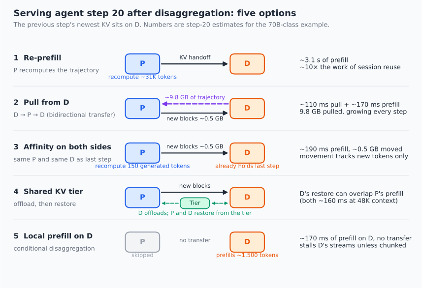
The five options side by side; each is explained below.
Option 1: Re-prefill. P recomputes everything after the shared prefix. This is the “shared prefix only” row in Section 5: correct and simple, but about 3.1 seconds of prefill at step 20 and about 10× the prefill work of real session reuse.
Option 2: Pull from D (D → P → D). P fetches the session’s KV from D, computes only the new tokens, and D then fetches the new blocks from P. vLLM implements this as bidirectional KV transfer (NixlConnector guide):
- A stateful proxy tracks sessions by a
conversation_idin the request body, a non-standard extension to the OpenAI API that the proxy consumes. - At the end of each turn, D returns its own transfer parameters, and the proxy caches them.
- On the next turn, the proxy attaches D’s block IDs to the request it sends to P. P pulls those blocks over RDMA before prefilling only the new tokens, and D then pulls the new blocks from P.
| Setting | Default | Meaning |
|---|---|---|
bidirectional_kv_xfer | false | Enables D → P pulls; must be set on both P and D |
kv_recompute_threshold | 64 tokens | Below this many remote tokens, P recomputes instead of pulling |
decoder_kv_blocks_ttl | 480 s | How long D keeps a finished turn’s blocks for reuse; not extended by heartbeats |
The catch for long agent sessions is that the amount pulled grows with the session. Suppose step 20 lands on a P worker that holds only the shared prefix. D holds everything up to and including its last tool call, so P must pull about 30,000 tokens of trajectory: 9.8 GB, or about 110 ms over two 400 Gb/s NICs. P then prefills only the 1,500-token tool output, which takes about 170 ms. The bytes moved per step grow linearly with session length, while the new work per step grows only slowly. Over NVLink the pull costs about 5 ms and barely matters. Over 400 Gb/s RDMA it adds about two-thirds of the prefill time to the step, and that fraction keeps growing as the session lengthens.
Option 3: Affinity on both sides. Route step k+1 to the same P and the same D that served step k.
- On P, the local prefix cache already covers everything P prefilled for step
k. It is missing only D’s 150 generated tokens, which cost about 17 ms to recompute because they attend over a 62,000-token context. - On D, the local cache already holds the entire previous sequence, so D loads only the blocks for the new tool output, about 0.5 GB, provided its connector loads only tokens beyond its local prefix-cache hit.
Both engines find their reusable blocks through their own content-hashed prefix caches, so this option needs no new mechanism beyond affinity routing and connectors that respect local hits. Data movement per step now tracks new tokens, not session length. The price is that P’s memory doubles as a session store and must be sized for it, and that affinity constrains load balancing, just as it does in a co-located deployment.
One exception matters a lot. When the generated tokens are a long reasoning trace that stays in the history, recomputing them is expensive: about 760 ms for an 8,000-token trace generated at around 40,000 tokens of context, versus about 29 ms to transfer its 2.6 GB over two 400 Gb/s NICs. In that case, pulling the generated span from D is worth it even under affinity, subject to the alignment check described below.
Option 4: A shared tier. D writes session KV to host memory or a distributed store as it decodes, and the next step’s P and D restore it from there. Neither side then needs to hold the session in HBM during the tool call. SGLang supports asynchronous KV offload from decode nodes in PD mode (--disaggregation-decode-enable-offload-kvcache), so later turns can find the KV in the shared tier (HiCache best practices).
Disaggregation also creates a useful overlap here. If the router picks the D worker as soon as the step arrives, rather than after prefill finishes (Mooncake’s scheduler, for example, selects the prefill–decode pair up front), D can restore a 48,000-token session from host memory over PCIe while P prefills the step’s new tokens. Both take about 160 ms, so the restore hides behind work that had to happen anyway.
Option 5: Prefill the increment locally on D. This is conditional disaggregation (Section 7) applied to sessions. If step 20 lands on the decode worker that still holds the session, its effective prompt length is about 1,500 tokens, below Dynamo’s default 2,048-token threshold, and only about 2% of the 63,000-token raw prompt, so the default policy serves it locally. That local prefill is roughly 170 ms of compute, which would stall D’s other streams unless chunked, reintroducing the co-located trade-off. It is a good option when D is lightly loaded and a poor one when D is full; Dynamo’s optional decode-busy guard covers part of that by reverting to remote prefill when the decode worker’s KV usage is too high.
9.3 Recompute or transfer: where the crossover really lies
vLLM’s default rule for D → P pulls, “recompute below 64 tokens,” is a sensible starting point, but the real crossover depends on two things the rule ignores.
Context length. Recomputing a token costs its share of the weight FLOPs plus attention over the entire preceding context. At the example’s step-20 context, recomputing 150 tokens takes about 17 ms. Transferring their 49 MB takes about 0.5 ms, plus fixed per-transfer costs; an example in vLLM’s documentation shows an average posting time of about 0.7 ms. At long contexts, even short tails are worth transferring. At short contexts, recomputing is cheaper.
P’s load. An idle P running a small prefill is bound by weight streaming: a pass costs about the same ~9 ms whether it carries 20 tokens or about 150 (the crossover at 60% of peak compute), so extra tokens up to that point are nearly free. A P already saturated with batched prefill work pays full compute price for every extra token.
A threshold that accounts for context length and P load will beat any fixed token count.
9.4 The correctness trap: content- vs. position-addressed reuse
The options above differ in how they find reusable KV:
- Affinity (option 3) relies on each engine’s own content-hashed prefix cache, so it is safe by construction.
- Pulls keyed by session (option 2, and the reasoning-trace pull in option 3) are position-addressed. They attach another engine’s blocks by position, assuming the new prompt extends the stored sequence token for token.
The history edits listed in Section 5 merely cause cache misses in content-addressed schemes. In position-addressed schemes they cause wrong output: the model attends to KV computed for different tokens, with no error raised. vLLM’s documentation calls out one such case directly. With reasoning models, D’s blocks cover the full generated sequence, including the <think> trace. When the client strips the trace from the history, the prompt P receives is missing tokens from the middle of D’s sequence, so pulling D’s blocks transfers KV for the wrong positions and produces incorrect output (vLLM issue #43094). The documentation currently assumes the router can detect such mismatches.
Rule of thumb. A router should verify token-level agreement before it attaches any remote blocks, for example by comparing block hashes computed over D’s token IDs with those of the new prompt.
10 From analysis to deployment: sizing the pools and deciding whether to split
10.1 Sizing P and D for the agent workload
A first-order model sizes P by throughput and D by Little’s law, which says the average number of items in a system equals their arrival rate times the time each spends there:
The D pool must satisfy two limits, and needs whichever is larger:
The scenario. The team runs 60 concurrent agent sessions on one repository. A step’s cycle is about 0.16 s of prefill, then 150 output tokens at a 25 ms TPOT target (3.75 s), then about 4 s of tool execution. That works out to roughly 7.6 agent steps per second across the fleet, with an average session context of about 48,000 tokens. All P estimates below assume this same step rate.
| Quantity | Estimate |
|---|---|
| P instances needed, full session reuse | ~1.2 |
| P instances needed, shared-prefix hits only (trajectory recomputed each step) | ~11 |
| P instances needed, no caching | ~28 |
| Concurrent decodes (7.6 steps/s × 150 tokens × 25 ms) | ~28 |
| D capacity if all 60 sessions stay warm in HBM (BF16, ~15.7 GB each) | ~940 GB, about 5 instances |
| Same, FP8 KV | about 2.4 instances |
| Same, BF16 with the shared prefix deduplicated on D | about 1.7 instances |
| D capacity if only sessions that are decoding or about to decode stay in HBM (idle ones offloaded) | ~470 GB, about 2.3 instances |
| Decode step, two D instances with ~14 decoding sessions each | ~23 ms with standard paged attention; ~14 ms with a cascade kernel |
| Decode step, one D instance holding all ~30 active sessions (BF16, prefix deduplicated, idle sessions offloaded; ~170 GB of KV) | ~37 ms with standard paged attention, missing the 25 ms target; ~19 ms with a cascade kernel |
Four lessons fall out of this table.
- Caching strategy moves the P pool by more than an order of magnitude. Session reuse versus prefix-only reuse is the difference between about one P instance and about eleven, which no amount of P-side kernel tuning can match. Because session reuse shrinks P demand without shrinking D residency, cache-heavy workloads push the optimal P:D ratio toward D.
- For agents, the D pool is sized by KV residency, not decode compute. Only about 28 sequences are decoding at any instant, but up to 60 sessions want their KV kept warm through tool calls. FP8 KV and offloading idle sessions each roughly halve the D pool, and deduplicating the shared prefix cuts it by nearly two-thirds.
- Offloading idle sessions can be nearly free under disaggregation. As Section 9 showed, the ~160 ms restore can hide behind P’s prefill of the new tool output.
- Deduplication fixes capacity; only a cascade kernel fixes bandwidth. The last row shows it: the consolidated instance fits in memory but misses the TPOT target unless its attention kernel reads the shared prefix once per step.
10.2 The same agent on an MLA mixture-of-experts model
Everything so far used a 70B dense model with GQA. Rerunning the key numbers for a DeepSeek-V3-class mixture-of-experts model with MLA shows which conclusions depend on the model:
| Quantity | 70B dense, GQA (running example) | DeepSeek-V3-class MoE with MLA |
|---|---|---|
| Parameters active per token | ~70.6B | ~37B |
| KV per token (BF16) | 320 KiB | ~68.6 KiB |
| Step-20 session KV (63,450 tokens) | ~20.8 GB | ~4.5 GB |
| Prefill compute for the 32,100-token first request | ~5.9 × 10¹⁵ FLOPs | ~5.0 × 10¹⁵ FLOPs |
| Share of that prefill compute spent in attention | ~23% | ~52% |
| KV handed off for that request | ~10.5 GB | ~2.3 GB |
| KV under tensor-parallel attention | sharded by KV head | replicated on every GPU |
| Decode attention intensity | ~8 FLOPs/byte | ~240 FLOPs/byte (all 128 heads on one GPU) |
- The handoff gets much cheaper relative to prefill. KV per token is about 4.7× smaller, but prefill compute barely drops. Prefill usually runs MLA in its expanded form, with 128 heads of 192-dimensional queries and keys and 128-dimensional values, so attention is about half the work despite the smaller active parameter count. The handoff’s share of prefill time ends up about 4× smaller than in the dense example, which is why MLA models sit at the friendly end of the table in Section 8.3.
- The parallelism layout decides whether smaller KV means more sessions. Under tensor-parallel attention, every GPU stores every sequence’s latent, so an 8-GPU node holds only as many sessions as a single GPU’s KV budget allows. Data-parallel attention, where each GPU attends only for its own sequences, recovers up to 8× more session capacity. This is one reason MLA models are usually served with data-parallel attention, as DeepSeek does in both phases (Section 7.1).
- Decode attention is no longer purely memory-bound. At about 240 FLOPs per byte, absorbed MLA decode sits near the ridge point (Section 2.3). Halving its KV bytes with FP8 would push it past the ridge if the attention math stays in BF16, so beyond that point smaller KV formats buy capacity rather than decode speed.
10.3 Co-located or disaggregated: a checklist
Stay co-located when most of these hold:
- the fleet is small, and operational simplicity matters more than peak utilization;
- prompt and output lengths are fairly stable;
- chunked prefill already keeps tail TPOT within its target;
- there is no low-latency, high-bandwidth path between machines (RDMA or NVLink);
- cache-aware routing, a cluster-wide KV index, and a plan for transfer failures are not yet in place;
- most traffic is multi-turn or agentic, and turns cannot yet be routed back to the workers or shared tier that hold their KV.
Consider disaggregating when several of these hold:
- long prompts (documents, repositories, agent histories, large tool schemas) regularly make prefill heavy;
- decode-side TPOT jitter is visible to users or downstream systems;
- the ratio of input to output work shifts enough that pools should scale separately;
- prefill and decode would benefit from different parallelism or hardware;
- P and D can share an NVLink domain or a well-provisioned RDMA fabric, and transfers and cache hits can be observed end to end.
10.4 Measuring each stage of TTFT
In a disaggregated system, TTFT is a sum of stages:
Instrument each term separately. Recent vLLM versions export per-transfer histograms for NIXL (vllm:nixl_xfer_time_seconds, vllm:nixl_post_time_seconds, vllm:nixl_bytes_transferred, vllm:nixl_num_descriptors) along with counters for failed transfers and expired leases. Common patterns:
| Symptom | Likely cause | First thing to try |
|---|---|---|
| Transfer P90 far above the average | Congestion or straggler links | Check NIC rail and topology placement; keep P and D in the same NVLink or leaf domain |
| High posting time, low transfer time | Many small descriptors from fragmented blocks | Use larger blocks or a more contiguous KV layout |
| Expired leases climbing | Lease too short for the network or workload, or D stopped heartbeating (aborts, network faults) | Lengthen kv_lease_duration; check D health and the network path |
| TTFT rising while prefill time is flat | D admission waits for free KV blocks | Add D capacity, use FP8 KV, offload idle sessions, deduplicate shared prefixes |
| Low prefix hit rate despite shared prompts | Volatile tokens early in the prompt, or cache-unaware routing | Reorder the prompt from stable to volatile; enable KV-aware routing |
| Session reuse rate low for agents | Turns land on different P or D workers, or blocks are evicted during tool calls | Add session affinity, a shared tier, or a longer decode-side TTL |
Takeaway. Size P by prefill throughput after caching and D by KV residency; caching choices move both pools far more than kernel tuning does.
11 Looking ahead: more splits and KV as a cluster resource
More disaggregation axes. The idea of splitting work by resource profile and then moving state between pools keeps spreading:
- Encode–prefill–decode. Multimodal serving separates the vision encoder into its own stage. SGLang supports this with Mooncake as the transfer backend, and vLLM documents a disaggregated encoder.
- Attention–FFN disaggregation. For MoE models, attention and expert FFNs can run on separate GPU groups, with micro-batches shuttled between them every layer. MegaScale-Infer reported up to 1.90× higher per-GPU throughput with this design (paper). Later analyses suggest the benefit depends heavily on interconnect bandwidth and expert granularity.
KV as a first-class cluster resource. Mooncake’s architecture puts the KV cache at the center of scheduling. Its scheduler moves reusable KV to the chosen prefill instance, streams new KV to decode, and rejects requests early under overload rather than degrading everyone’s latency. The authors report that this design let Kimi handle 75% more requests under real workloads (Mooncake, FAST ‘25). The tiered stores from Section 5 share this direction: KV lives in a cluster-wide, multi-tier store, and placement decisions follow it.
Hardware pushes toward overlap and smaller KV. Because per-GPU compute has recently grown faster than per-GPU scale-out bandwidth (Section 8), three responses are gaining ground: streaming the transfer so it hides behind prefill, shrinking the KV itself (FP8 or 4-bit formats, MLA-style compression, sparse attention), and keeping P and D inside one rack-scale NVLink domain so the handoff becomes a local copy rather than a network transfer.
12 Conclusion: get the cache design right first
The three caches are three different kinds of things:
- The KV cache is data: the keys and values every token produced at every layer.
- The prefix cache is a content policy: if two prompts start with the same tokens, they can share the same blocks.
- The session cache is an identity and lifecycle policy: which conversation owns which blocks, where they wait between turns, and how they come back.
In a co-located server, all three live in one block pool, and the hard problem is scheduling prefill and decode on the same GPUs. Disaggregation removes that problem by separating where tokens are computed. In exchange, it turns all three caches into distributed-systems questions: which machine holds the prefix, which holds the newest copy of a session, and whether moving the state is cheaper than recomputing it.
Takeaway. For long-context and agentic workloads, caching decisions (session reuse, affinity, tiering, KV format, prefix deduplication) determine how much traffic a given fleet can serve far more than the choice between co-located and disaggregated serving does. Get the cache design right first, then decide where to split.
References
- vLLM: Automatic Prefix Caching design
- vLLM: NixlConnector usage guide (pull mode, bidirectional KV transfer, failure policy, metrics)
- vLLM: NIXL push-mode KV transfer design
- vLLM: KV connector API (
KVConnectorBase_V1) - FlashInfer (including cascade attention for shared prefixes)
- NVIDIA Dynamo: Routing concepts
- NVIDIA Dynamo: Conditional disaggregation
- NVIDIA Dynamo: KVBM configuration reference
- SGLang HiCache (LMSYS blog)
- SGLang HiCache best practices
- DistServe: Disaggregating Prefill and Decoding for Goodput-optimized LLM Serving (OSDI ‘24)
- Splitwise: Efficient Generative LLM Inference Using Phase Splitting (ISCA ‘24)
- Sarathi-Serve: Taming Throughput-Latency Tradeoff in LLM Inference (OSDI ‘24)
- Mooncake: A KVCache-centric Disaggregated Architecture for LLM Serving (FAST ‘25)
- MegaScale-Infer: Serving Mixture-of-Experts at Scale with Disaggregated Expert Parallelism
- DeepSeek-V3/R1 Inference System Overview
- OpenAI: Prompt caching
- NVIDIA: Introducing NVFP4 for efficient and accurate low-precision inference
A note on the numbers. All latency, capacity, and sizing numbers are estimates derived from the stated model and hardware assumptions (60% of peak dense BF16 for prefill; effective link bandwidths as listed). Capacity decisions should rest on measurements from the target stack.